Dayname (Non-English Version)

Category: Multiple Formulas
Level: Intermediate

Unfortunately, Ms Excel just support English in date format compared with OpenOffice.org (OOo) Calc. So, you can’t perform the previous tips of Dayname (English Version) if you want to use another language. This weakness makes us more creative to create multiple formulas.

We will take the advantages of CHOOSE and WEEKDAY formulas.

CHOOSE(index_num, value1, value2, ...)
Index_num specifies which value argument is selected. Index_num must be a number between 1 and 29, or a formula or reference to a cell containing a number between 1 and 29.
If index_num is 1, CHOOSE returns value1; if it is 2, CHOOSE returns value2; and so on.

WEEKDAY(date, type)
type 1 or omitted return integer 1-7, where 1 for Sunday and 7 for Saturday
type 2 return integer 1-7, where 1 for Monday and 7 for Sunday
type 3 return integer 0-6, where 0 for Monday and 6 for Sunday

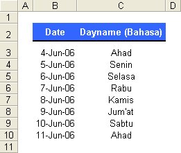
This example shows how to get dayname in Bahasa.



Using same case with previous posting, Dayname (English Version), use this formula in cell of C3:
=CHOOSE(WEEKDAY(B3),"Ahad","Senin","Selasa",
"Rabu","Kamis","Jum'at","Sabtu")

Dayname (English Version)

Criteria: Technical, Multiple Formulas
Level: Intermediate

I myself often face this problem. That is, what is the dayname of certain date. Before found this multiple formulas from my partner job, Michael HTj, I always use macro. What a stupid way! Thx Mike! Now, I want to share how to get dayname of certain date.

There are two ways to have it:

.: Using format cell

1 Right click on selected range
2 Chose Format Cells...
3 In Number tab, chose Custom
4 Type ddd or dddd in Type textbox
5 To see the result, see in Sample box
6 OK



.: Using TEXT formula

TEXT(value, format_text)
Value is a numeric value, a formula that evaluates to a numeric value, or a reference to a cell containing a numeric value.
Format_text is a number format in text form from in the Category box on the Number tab in the Format Cells dialog box. Format_text cannot contain an asterisk (*) and cannot be the General number format.

For this case, set format_text to ddd for simple day (e.g. Sun) or dddd for complete day (e.g. Sunday)



Here are the formulas in cells of C3 and D3:
=TEXT(B3,"ddd")
=TEXT(B3,"dddd")
respectively.

SUMIF Formula

Catogory: Bulit-in Formula
Level: Beginner

This is request formula from Miss Sri. How to use SUMIF formula?

SUMIF is a built-in formula in Excel. It means, that u don't have to make it by yourself. U just use it and u have to know how to use it. Actually, you can read it in Ms Excel's Help? And I think the Help is helpfull enough. But less application to the case.

SUMIF(range, criteria, sum_range)
Range is the range of cells you want evaluated.
Criteria is the criteria in the form of a number, expression, or text that defines which cells will be added. For example, criteria can be expressed as 32, "32", ">32", "apples".
Sum_range are the actual cells to sum. The cells in sum_range are summed only if their corresponding cells in range match the criteria. If sum_range is omitted, the cells in range are summed.

OK. I will use the data from the previous posting, AVERAGEIF Formula. The goal is to find the sum of each subject.



U just put these formulas in cell of D16, D17, and D18:
=SUMIF($C$3:$C$13,C16,$D$3:$D$13)
=SUMIF($C$3:$C$13,C17,$D$3:$D$13)
=SUMIF($C$3:$C$13,C18,$D$3:$D$13)
respectively.

There is other ...IF formula: COUNTIF

Generating Normal Distribution Data

Category: Built-in Formula
Level: Intermediate

If u are a statistician or a researcher, this tip must be very important. Generating normal distribution data in Excel is very easy. Using formula NORMINV, u can get the data following normal distribution.

NORMINV(probability, mean, standard deviation)
Returns the inverse of the normal cumulative distribution for the specified mean and standard deviation.
Probability is a probability corresponding to the normal distribution.
Mean is the arithmetic mean of the distribution.
Standard deviation is the standard deviation of the distribution.

For example, I want to generate 50 data following normal distribution with mean 100 and Standard Deviation 5.

Put the parameters in E5 for mean and E6 for standard deviation
Write this formula in range B8:F17
=NORMINV(RAND(),$E$5,$E$6)



And tada…. U can check the accuracy of mean and standard deviation using AVERAGE and STDEV formula. See cell of E21 and E22.

AVERAGEIF Formula

Category: Multiple Formulas
Level: Intermediate

Excel has a formula to count sum with any condition, SUMIF. But there isn't built-in formula to count average with any condition, e.g. said AVERAGEIF. Then u yourself must write function with macro. But any other solution without macro?

The anwser is absolutly.... yes! *Horrayy*
U can use the advantage of array function, which is by pressing Ctrl+Shift+Enter after u write the formula. Then u can see that the formula shows in the bracket {..}.

The formula is
=AVERAGE(IF(array of condition = condition, array of average))
and followed by pressing Ctrl+Shift+Enter

For example. This table below shows the rate of subject by student. Our mission is find the average of each subject.



U just write the formula in D16, D17, and D18, respectively:
=AVERAGE(IF($C$3:$C$13=C16,$D$3:$D$13))
=AVERAGE(IF($C$3:$C$13=C17,$D$3:$D$13))
=AVERAGE(IF($C$3:$C$13=C18,$D$3:$D$13))
and don't forget to press Ctrl+Shift+Enter.

2D lookup

Category: Multiple Formulas
Level: Intermediate

Are u ever use vlookup or hlookup formula?
These formulas just can search a cell with a criteria. Then what should we do if we have 2 criterias?

It's simple u can use this formula
=INDEX(table, MATCH(column criteria, first column of table, 0),MATCH(row criteria, first row of table, 0))

For example, I have a table. First row is subject name and first column is student name. I want to know what is Udin's rate in Basic Mathematic subject.



The formula in C11 is:
=INDEX(B2:E8,MATCH(B11,B2:B8,0),MATCH(C10,B2:E2,0))

Welcome

Assalaamu'alaykum.



Begin from this day, I'll post about some tips in using Microsoft Excel.
I hope, this blog usefull for all Excel users.
If any questions then u can write it in shoutbox.

Best Regards.